How spatial intelligence and tagging show where research is missing

What spatial intelligence means here

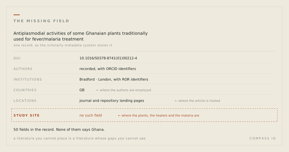
Spatial intelligence is a machine reasoning about where things are and how places relate: which points fall inside which region, how far one thing is from another, what clusters and what is absent. The scientific record has given it almost nothing to work with: as we set out in the missing field, no metadata field records where a study happened; the only location carried is the authors’ employer.

So for COMPASS ID spatial intelligence begins by making the missing field. We read the study site out of the paper’s own text and resolve the place name to coordinates through a gazetteer, which is a dictionary of place names with their locations. That step is called geoparsing. Only sites from a fixed list of trusted geocoding sources count, an author’s address never does, and a paper whose site cannot be resolved with confidence is flagged as unlocated rather than guessed. Then the reasoning starts: which species have been studied inside their own range, where research clusters and where it is absent, how far from a city or a station fieldwork happens, and what a given place knows about itself.

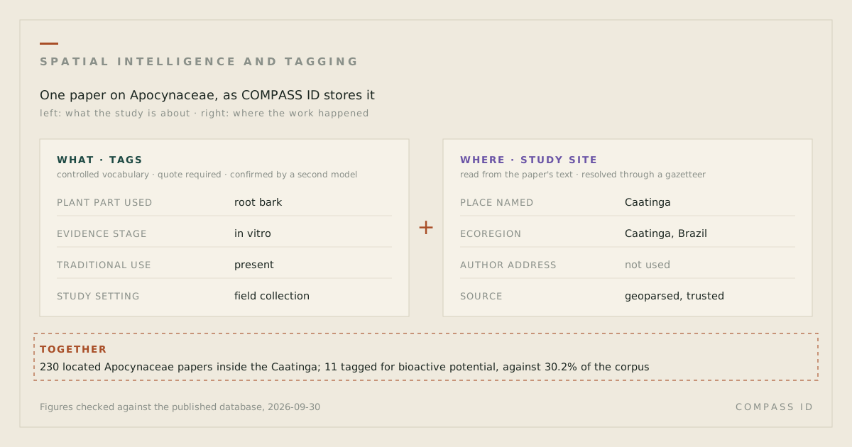
Tagging is the other half, and spatial intelligence is not much use without it. A model reads the paper and assigns values from a controlled vocabulary, meaning a fixed list of dimensions and allowed values written by people who know the field, such as the plant part used, the stage of pharmacological evidence reached, or the policy framework named. A tag is kept only when it cites a passage in the paper and a second model, given the same rubric, confirms it. Tags say what. The place says where. The paper joins them.

What tags and places each measure on their own

Tags alone produce a very good bibliography. They can say that a family’s literature is mostly chemistry, and nothing about whether any of it was done where the plants grow. Place alone is a map of dots. It shows clusters, but not what the clustered papers are about, and it cannot tell a field survey from a laboratory screen that happened to name a collection site. Spatial intelligence over a tagged corpus gives the dots subject matter and the subjects an address.

Study sites compared with species ranges

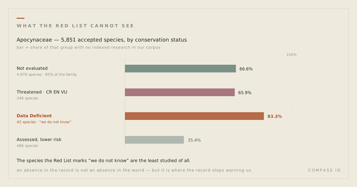
The first question: has each species been studied where it lives? Apocynaceae, the dogbane and milkweed family that gave medicine vincristine and reserpine, has 6,759 accepted species in our census. 4,292 of them have no indexed research. Of the 2,467 that do, 1,198 have papers but no locatable study site anywhere: the work exists, and it happened somewhere the text does not name, usually a laboratory.

Now take the 6,753 species for which the Kew World Checklist of Vascular Plants, Version 16, the same checklist the census comes from, records the countries of the native or introduced range. Only 1,185 of them, 17.5 percent, have a located study site inside one of those countries. Put the other way, 5,568 species with a known range, 82.5 percent, have no located study inside it. This is a country-level test and a generous one: a study in a botanic garden in the right country counts as in range, and the range list includes countries where the species is only introduced.

The same reasoning runs by country. 435 census species have Venezuela among their range countries. 8 of them have a located study site in the country; 427 do not. The whole 33,900-paper corpus holds 7 study sites that could be placed in Venezuela at all, and one of the 7 resolves only to the country itself. A tag count would have said the family is well studied. It is. The place count says where it has not been.

Study sites compared with research stations

The second question is distance. Antarctica turns the range question around: there the research is located, but in the same few places. The corpus has 5,550 papers, and 3,967 of them name a locatable study site, a far higher share than the plant literature because Antarctic science is largely fieldwork. Set aside country centroids and other imprecise placements and those papers resolve to 462 precise sites. Measured against the research stations listed by COMNAP, the Council of Managers of National Antarctic Programs, the median site is 125.9 km from the nearest station and 45.2 percent lie within 100 km of one. McMurdo (United States) and Scott Base (New Zealand), which sit side by side on Ross Island, each have 73 sites within 100 km; Mario Zucchelli (Italy) has 44. These are straight-line distances, not travel times.

For the plant family the equivalent access point is a city rather than a station: the median study site is 46.9 km from a city of 100,000 people or more, and 91.9 percent lie within 200 km of one. Fieldwork happens where it can be reached, and a hard-to-reach species or region is under-represented before anyone has judged it unimportant.

Study sites within one ecoregion, the Caatinga

The third question starts from a place rather than a species: the place explorer lets you pick one and see what has been studied inside it, and how that mix compares with the whole field. Take the Caatinga, the dry forest of north-eastern Brazil. It is an ecoregion, meaning a region defined by its characteristic plants and animals; we use the RESOLVE 2017 set of 847 ecoregions. Of the 4,625 Apocynaceae papers with a located study site anywhere, 230 have one inside the Caatinga, more than any other ecoregion.

Now compare the tags on those 230 papers with the tags on the whole corpus. Across all 33,900 papers, 30.2 percent (10,232) carry a bioactive-potential tag, 31.2 percent (10,572) a compound class, and 43.8 percent (14,840) a pharmacological evidence stage. Inside the Caatinga the same three dimensions run at 4.8 percent (11 of 230), 5.7 percent (13 of 230) and 10.4 percent (24 of 230). The explorer flags a dimension as thin when its share inside a place falls below half its share in the corpus; these sit at a sixth to a quarter.

That says two things at once, and the page prints both denominators so that a reader can hold them apart. The located Caatinga literature on this family is ecology and ethnobotany, not chemistry: the ecoregion with the most located research on the family carries almost none of its drug-discovery work. And chemistry papers seldom name a field site at all, so the located subset of any place leans toward fieldwork. The first is a fact about the Caatinga; the second is a fact about the record, and it is why every inside count on that page is stated as a lower bound. This finding needs both halves: spatial intelligence draws the boundary and finds the papers inside it; only the tags say what they are about.

Study sites compared with land change

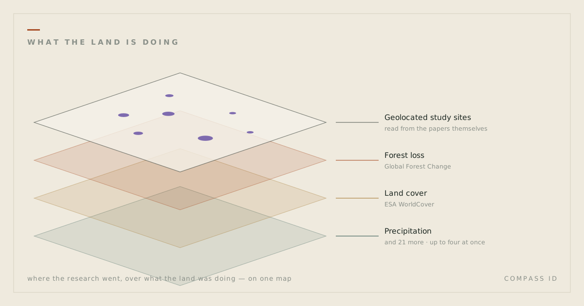
The fourth question sets the same study sites against the environment changing around them. Three change layers were read from Earth observation products for every hexagonal cell and for 847 ecoregions and 3,686 first-level administrative regions: forest loss from 2001 to 2024, the trend of the aridity index from 1990 to 2024 and, for Antarctica, the sea-ice trend. Each unit was placed in a quadrant by its rate of change and by the density of located research inside it.

The first result is an absence. Across the Apocynaceae corpus, Spearman’s rank correlation between forest loss and located research density is −0.013 across 532 ecoregions and 0.000 across 1,846 administrative regions. Research effort does not track environmental change in either direction. That is a descriptive figure, not a cause: units differ in area, access and richness. The second result is the list it leaves behind: 68 of those 532 ecoregions are in the top third for forest loss and have no located Apocynaceae paper at all. Peninsular Malaysian peat swamp forests lost 58.0 percent of their 2000 forest and have 393 range species of the family with no study site inside them. Forest loss in this product includes plantation harvest, so the list is a prompt to check, not a verdict. The third result is time: 77.9 percent of the located Apocynaceae research was published in the 2010s or 2020s, against 67.5 percent of the whole corpus, so the located record is the recent record.

Expected research (beta)

The fifth question turns the map around: given what we know about a place, how much located research would it be expected to have? A model in beta fits that expectation for every ecoregion and administrative region from species richness, distance to the nearest large city, forest loss and aridity trend, biome and national research effort, with area as exposure, so a larger unit is expected to carry more papers. Observed minus expected is the residual, and a place with less than expected is a candidate gap, never proof of neglect: the model predicts where research tends to go, not where it is needed.

Fit is measured on whole realms and countries held out of the fit. That cross-validated pseudo-R2, the share of variation explained in places the model has not seen, is 0.63 for Apocynaceae ecoregions and 0.48 for administrative regions; for the desertification corpus it is 0.49 and 0.44. The Purus-Madeira moist forests have 0 located Apocynaceae papers against 15.99 expected, with a 90 percent interval of 0 to 51; the Arabian sand desert has 0 against 14.96, interval 0 to 48. In the desertification corpus the North Tibetan Plateau-Kunlun Mountains alpine desert has 2 papers against 177.25 expected, interval 6 to 563, and Gafsa, in Tunisia, has 0 against 14.88, interval 0 to 52.

Located research is so clustered that these intervals are wide: no place in any atlas falls formally below its interval in this run, so the rankings order places by the tail probability, the chance of a count at or under the observed one given the expectation. The residuals also audit the geocoder: Sahel, a province of Burkina Faso, carries 109 desertification papers against 9.13 expected, above its interval of 0 to 32, likely a place-name collision with the Sahel region. See Expected research (beta) on any atlas, or the layer Expected vs observed on the interactive map.

What makes it auditable

Every number above is checked, not remembered. A figures audit re-derives each published figure from the database or the atlas data file on every run, and a page whose wording no longer matches its check fails the run. The numbers in this post were added to that manifest before publication, so they fail loudly rather than drift quietly as the census and the harvest grow. Every count carries a denominator, because 1,185 means nothing without the 6,753 it was drawn from, and the 6,753 means nothing without the 6,759 behind it.

The place layer states its own caveats on every page that uses it. Study-site coordinates come from automated geoparsing; a 40-site manual check found 31 plausible, and a larger human check is planned. Ranges are country lists from the Kew World Checklist of Vascular Plants, not distribution maps, so in-range is generous and outside-only is conservative. Distances are straight lines. And every blank reads no indexed research, never no research: an absence in an index is a statement about the index.

What comes next

The change layers and the decade split above are now on every atlas page, as the section Research against change, and on the interactive map as switchable layers with a decade selector. Two further pieces are being built. The first is marine units, so that the quarter of Antarctic study sites in open water can be set against a spatial unit rather than a cell alone. The second is protected-area status, so that a gap can be read against where protection already stands. Neither is published yet, and neither carries a number here. The third is a human check of the expected-research model, still in beta, against expert judgement: whether the places it ranks as candidate gaps are the ones people who know a family or a region would name, and whether the places it ranks above expectation are research clusters or geocoding errors.

What spatial intelligence adds

Tagging alone says what has been written. Spatial intelligence adds where: inside a range or not, how far from a station or a city, what a place holds and lacks, and, in beta, how much it would be expected to hold. Joined on the paper, the two show that in one plant family four species in five with a known range have no located study inside it, that nearly half of Antarctic study sites lie within 100 km of a station, that the ecoregion with the most located research on the family carries almost none of the family’s chemistry, and that where forest is being lost fastest is no guide to where the family has been studied. Those are measurements of an index, not of the world, and every one of them can be re-run.

Sources

• Dinerstein, E. et al. (2017). An Ecoregion-Based Approach to Protecting Half the Terrestrial Realm. BioScience 67(6): 534–545. doi:10.1093/biosci/bix014 (RESOLVE Ecoregions 2017, CC-BY 4.0)
• COMNAP (2024). Antarctic Facilities, v3.5.0. Council of Managers of National Antarctic Programs. comnap.aq/antarctic-facilities-information
• Govaerts, R. (ed.) (2026). WCVP: World Checklist of Vascular Plants, Version 16. Royal Botanic Gardens, Kew. Extracted 4 June 2026. doi:10.34885/egs6-cp24 (species census and distribution table, TDWG level-3 areas mapped to countries)
• Natural Earth. Populated places, 1:10m (places with 100,000 people or more). naturalearthdata.com
• Hansen, M.C. et al. (2013). High-Resolution Global Maps of 21st-Century Forest Cover Change. Science 342: 850–853. doi:10.1126/science.1244693 (Global Forest Change v1.12, 2001 to 2024, CC BY 4.0)
• Abatzoglou, J.T., Dobrowski, S.Z., Parks, S.A. & Hegewisch, K.C. (2018). TerraClimate, a high-resolution global dataset of monthly climate and climatic water balance from 1958–2015. Scientific Data 5: 170191. doi:10.1038/sdata.2017.191 (CC0)
• Huang, B. et al. (2021). Improvements of the Daily Optimum Interpolation Sea Surface Temperature (DOISST) Version 2.1. Journal of Climate 34: 2923–2939. doi:10.1175/JCLI-D-20-0166.1 (OISST v2.1 sea-ice field, public domain)
• Acheson, E. & Purves, R.S. (2021). Extracting and modeling geographic information from scientific articles. PLOS ONE 16(1): e0244918. doi:10.1371/journal.pone.0244918

Figures updated 3 October 2026 to the Kew WCVP Version 16 census (6,759 accepted species, 4,292 with no indexed research); see the atlas revision note.

See where the research is, and is not, on the Apocynaceae atlas →